Macroeconomic Data with Quantiacs
-
*This article was published on Medium: check it out here.
Quantiacs provides users with macroeconomic data from the U.S. Bureau of Labor Statistics. These data can be used on the cloud or downloaded locally for further analysis. In this article we show how to use macroeconomic data for developing a trading algorithm.
Bureau of Labor Statistics Data
The U.S. Bureau of Labor Statistics is the principal agency for the U.S. government in the field of labor economics and statistics. It provides macroeconomic data in several interesting categories: prices, employment and unemployment, compensation and working conditions and productivity.

Photo by Vlad Busuioc on UnsplashThe macroeconomic data provided by the Bureau of Labor Statistics are used by the U.S. Congress and other federal agencies for taking key decisions. They are very important data for academic studies. Moreover, they represent for quants an interesting source of ideas and can complement market data for developing trading algorithms.
Quantiacs has implemented these datasets on its cloud and makes them also available for local use on your machine.
Inspecting the Datasets
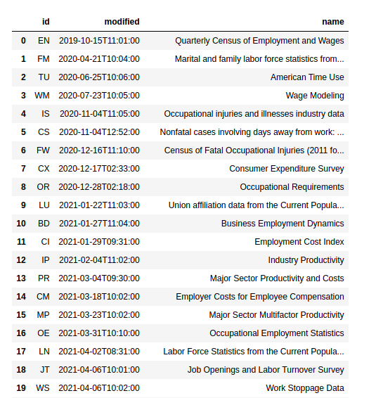
The data are organized in 34 datasets which can be inspected using:
import pandas as pd
import numpy as np

import qnt.data as qndata

dbs = qndata.blsgov.load_db_list()

display(pd.DataFrame(dbs))
The result is a table displaying the date and time of the last available update and the name of each dataset:
Each dataset contains several time series which can be used as indicators.
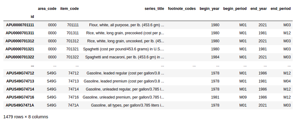
For this example we use AP, the dataset containing Average consumer Prices. They are calculated for household fuel, motor fuel and food items from prices collected for building the Consumer Price Index.Let us load and display the time series contained in the AP dataset:
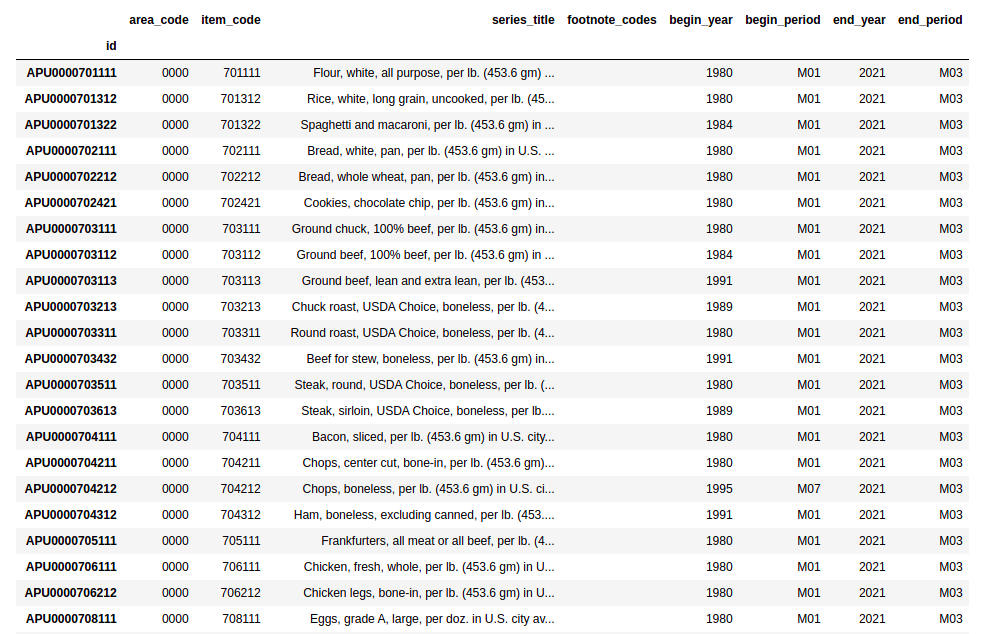
series_list = list(qndata.blsgov.load_series_list('AP'))

display(pd.DataFrame(series_list).set_index('id'))
The AP Average Price dataset contains 1479 time series, each with 8 different fields:
The meaning of some field for the time series is obvious:series_title, begin_year or end_year need no explanation. Other fields are not obvious at first glance, and their meaning should be inspected: this is the case for example of area_code, item_code, begin_period and end_period.
The meaning can be inspected using:
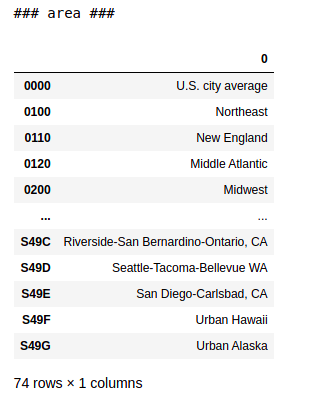
meta = qndata.blsgov.load_db_meta('AP')

for k in meta.keys():
    print('### ' + k + " ###")
    m = meta[k]

    if type(m) == str:
        # show only the first line if this is a text entry:
        print(m.split('\n')[0])
        print('...')
        # full text option, uncomment:
        # print(m)

    if type(m) == dict:
        # convert dictionaries to pandas DataFrame:
        df = pd.DataFrame(meta[k].values())
        df = df.set_index(np.array(list(meta[k].keys())))
        display(df)
The area_code column reflects the U.S. area connected to the time series, for example 0000 for the entire U.S.:
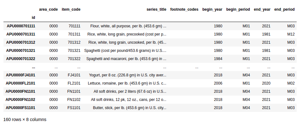
Let us select only time series related to the entire U.S.:
us_series_list = [s for s in series_list \
  if s['area_code'] == '0000']

display(pd.DataFrame(us_series_list).set_index('id'))
We have 160 time series out of the original 1479. These are global U.S. time series which are more relevant for forecasting global financial markets:
Let us select a subset of 55 time series which are currently being updated and have at least 20 years of history:
actual_us_series_list = [s for s in us_series_list \
    if s['begin_year'] <= '2000' and s['end_year'] == '2021' ]

display(pd.DataFrame(actual_us_series_list).set_index('id'))
The length of these time series is enough for backtesting trading ideas:
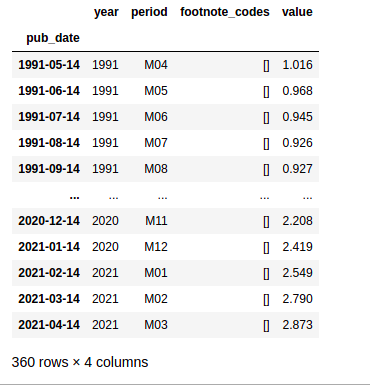
Now we can load one of these series and use it for our strategy. Let us focus on energy markets. We consider fuel oil APU000072511 on a monthly basis:
series_data = qndata.blsgov.load_series_data('APU000072511', \
              tail = 30*365)

# convert to pandas.DataFrame:
series_data = pd.DataFrame(series_data)
series_data = series_data.set_index('pub_date')

# remove yearly average data, see period dictionary:
series_data = series_data[series_data['period'] != 'M13']

series_data
and obtain one time series which can be used for developing a trading algorithm:
The Trading Algorithm

Photo by Maksym Kaharlytskyi on UnsplashWe focus on energy markets which we inspect using:
futures_list = qndata.futures_load_list()

energy_futures_list = [f for f in futures_list \
    if f['sector'] == 'Energy']

pd.DataFrame(energy_futures_list)
and obtain:
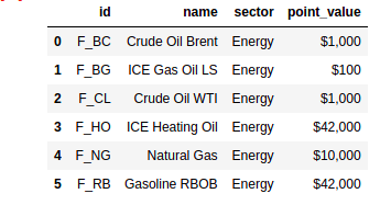
We use the Crude Oil WTI Futures contract, F_CL, and develop a simple strategy which uses fuel oil as an external indicator:
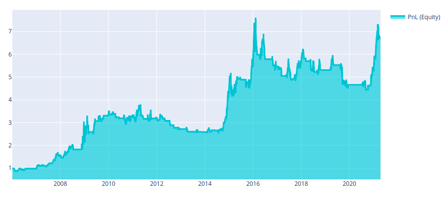
import xarray as xr
import numpy as np
import pandas as pd

import qnt.ta as qnta
import qnt.backtester as qnbt
import qnt.data as qndata


def load_data(period):

    futures = qndata.futures_load_data(assets=['F_CL'], \
             tail=period, dims=('time','field','asset'))

    ap = qndata.blsgov.load_series_data('APU000072511', tail=period)

    # convert to pandas.DataFrame:
    ap = pd.DataFrame(ap)
    ap = ap.set_index('pub_date')

    # remove yearly average data, see period dictionary:
    ap = ap[ap['period'] != 'M13']

    # convert to xarray:
    ap = ap['value'].to_xarray().rename(pub_date='time').\
      assign_coords(time=pd.to_datetime(ap.index.values))

    # return both time series:
    return dict(ap=ap, futures=futures), futures.time.values


def window(data, max_date: np.datetime64, lookback_period: int):
    # the window function isolates data which are
    # needed for one iteration of the backtester call

    min_date = max_date - np.timedelta64(lookback_period, 'D')

    return dict(
        futures = data['futures'].sel(time=slice(min_date, \
                  max_date)),
        ap = data['ap'].sel(time=slice(min_date, max_date))
    )


def strategy(data, state):

    close = data['futures'].sel(field='close')
    ap = data['ap']

    # the strategy complements indicators based on the
    # Futures price with macro data and goes long/short
    # or takes no exposure:
    if ap.isel(time=-1) > ap.isel(time=-2) \
            and close.isel(time=-1) > close.isel(time=-20):
        return xr.ones_like(close.isel(time=-1)), 1

    elif ap.isel(time=-1) < ap.isel(time=-2) \
            and ap.isel(time=-2) < ap.isel(time=-3) \
            and ap.isel(time=-3) < ap.isel(time=-4) \
            and close.isel(time=-1) < close.isel(time=-40):
        return -xr.ones_like(close.isel(time=-1)), 1

    # When the state is None, we are in the beginning
    # and no weights were generated.
    # We use buy'n'hold to fill these first days.
    elif state is None:
        return xr.ones_like(close.isel(time=-1)), None

    else:
        return xr.zeros_like(close.isel(time=-1)), 1


weights, state = qnbt.backtest(
    competition_type='futures',
    load_data=load_data,
    window=window,
    lookback_period=365,
    start_date='2006-01-01',
    strategy=strategy,
    analyze=True,
    build_plots=True
)
This strategy can be used as a starting point for improving (note that performance is positive, but In-Sample Sharpe ratio is smaller than 1 so the system should be improved for submission):
The source code is publicly available at our GitHub page and it can be found in your account at Quantiacs.
Do you have comments? Let us now in the Forum page!
-
@news-quantiacs
Thanks, well done!
How do you get 'state' though?TypeError Traceback (most recent call last) <ipython-input-1-8e93b849784e> in <module> 79 strategy=strategy, 80 analyze=True, ---> 81 build_plots=True 82 ) ~/book/qnt/backtester.py in backtest(competition_type, strategy, load_data, lookback_period, test_period, start_date, window, step, analyze, build_plots) 66 data, time_series = extract_time_series(data) 67 print("Run pass...") ---> 68 result = strategy(data) 69 if result is None: 70 log_err("ERROR! Strategy output is None!") TypeError: strategy() missing 1 required positional argument: 'state' -
@spancham
That's the new feature for sharing states between passes, you need to update your local quantiacs environment to use it. Took me some time to figure it out but what worked for me wasconda install quantnet::qnt@news-quantiacs
Thanks for the detailed explanation, it's indeed very helpful!
I stumbled across this dataset some time ago but got confused by its structure, now I can actually use it -
Thanks @antinomy!
That works. -
@spancham
You're welcome. However, there is a caveat: your old strategies won't work anymore.
One way of fixing it woud be to change the strategies. Let's say you have one that looks like this:def strategy(data): """ your code to calculate the weights here... """ return weightsThe updated baktester now expects your function to return 2 objects, the weights and the state (this can be anything like a dictionary, a number or even None but it has to be SOMETHING). So your strategy could look like this:
def strategy(data): """ your code to calculate the weights here... """ return weights, None(If you actually want to use the feature, take a look at the link in my previous reply)
Another way would be to dowgrade qnt again with
conda install quantiacs-source::qntYou could also make 2 envs, one with quantiacs-source::qnt for the old models and one with quantnet::qnt for the new ones...
-
This post is deleted! -
@antinomy
Thank you! -
This post is deleted!