Evaluation

Single-Pass Backtesting

This approach allows to evaluate your strategy very fast. It is very useful when you use any kind of optimization.

Often, single-pass strategies are looking forward. So it is necessary to test your strategy using multi-pass approach to avoid looking forward. It is possible to adapt multi-pass strategy for multi-pass backtester. See the files in the folder examples in the jupyter environment on the platform (or in the package qnt.examples).

Write Weights

The necessary input for backtesting is a set of allocation weights (fractions of capital to be invested) for all assets over the backtesting period. Let us suppose that we wrote the code:

import qnt.data as qndata
import qnt.ta as qnta

futures = qndata.futures.load_data(min_date="2006-01-01")

price_open = futures.sel(field="open")
price_open_one_day_ago = qnta.shift(price_open, periods=1)

strategy = price_open - price_open_one_day_ago

weights = strategy / abs(strategy).sum("asset")

Then we can submit code by importing in addition the qnt.output library:

import qnt.output as output

and a call to the write function:

output.write(weights)

Function

qnt.output.write(weights)

Parameters

Parameter	Explanation
weights	xarray.DataArray with allocation weights for all assets in the backtesting period.

Output

None, the call is mandatory as it will write weights to file used for evaluating performance.

Clean Weights

We provide you with a clean function which can be used for performing sanity checks on the defined weights. The function can be called before writing:

weights = output.clean(weights, futures, "futures")

It will perform 2 operations:

1. if there are trading days where the user did not specify any exposure, an exposure of “0” (no allocation) will be used;

2. if the total sum of the absolute exposure is larger than 1, normalization to 1 will be applied (i.e. max. allowed leverage is 1).

Function

qnt.output.clean(weights, data, kind)

Parameters

Parameter	Explanation
weights	xarray.DataArray with allocation weights for all assets in the backtesting period.
data	xarray.DataArray with input data.
kind	"futures" or "crypto".

If kind=”crypto”, the code will check in addition if other futures in addition to Bitcoin are defined. In positive case, it will remove them and leave Bitcoin futures only.

Output

An xarray.DataArray with the cleaned weights ready for submission.

Check Weights

In addition to the clean function we provide a check function which will return you warnings if issues with weights are present. The function can be called before writing:

output.check(weights, futures, "futures")

The first check is connected to the possible presence of missing values in your algorithm. With the previous call to the clean function, this problem is automatically solved.

The second check computes the In-Sample Sharpe ratio of your system. The In-Sample Sharpe ratio must be larger than 1 for a successful submission.

The third check controls correlation with existing templates and with all systems submitted to previous contests.

Function

qnt.output.check(weights, data, kind)

Parameters

Parameter	Explanation
weights	xarray.DataArray with allocation weights for all assets in the backtesting period.
data	xarray.DataArray with input data.
kind	"futures" or "crypto".

If kind=”crypto”, the code will check in addition if other futures in addition to Bitcoin are defined.

Output

None, only warning messages will be displayed.

Multi-Pass Backtesting

We provide you with a function for performing an optional backtesting which explicitely forbids looking-forward issues with a multi-pass implementation where at timestamp “t” only data until timestamp “t” are available by construction. It can be used with:

import xarray as xr
import qnt.ta as qnta
import qnt.backtester as qnbt
import qnt.data as qndata


def load_data(period):
    return qndata.futures_load_data(
        assets=["F_AD", "F_BO", "F_BP", "F_C"],
        tail=period)


def strategy(data):
    close = data.sel(field="close")
    sma_long  = qnta.sma(close, 200).isel(time=-1)
    sma_short = qnta.sma(close,  40).isel(time=-1)
    pos = xr.where(sma_short > sma_long, 1, -1)
    return pos / abs(pos).sum("asset")


weights = qnbt.backtest(
    competition_type = "futures",
    load_data        = load_data,
    lookback_period  = 365,
    test_period      = 365 * 15,
    strategy         = strategy)

Note that multi-pass backtesting is considerably slower than single-pass one. We suggest you to start with a simple single-pass implementation and to cross-check your results with the multi-pass implementation before submission, to get a realistic estimate of the performance of your algorithm.

Function

qnt.backtester.backtest(competition_type, load_data, lookback_period, test_period, strategy)

Parameters

Parameter	Explanation
competition_type	"futures" or "crypto".
load_data	data load function which returns data time series, accepts tail argument.
lookback_period	calendar days, max. lookback period for building indicators.
start_date	start date for backtesting, overrides test period
end_date	end date for backtesting, by default - now
test_period	calendar days, period used for the simulation.
strategy	strategy function, accepts data and returns weights for all assets for the last day.

Output

It returns the xarray.DataArray of weights and performs automatically calls to clean, check and write.

Stateful Multi-pass Backtesting

If you want to pass the state between iterations using the multi-pass backtesting, you can do it this way:

import xarray as xr
import numpy as np

import qnt.backtester as qnbt


def strategy(data, state):
    close = data.sel(field="close")
    last_close = close.ffill('time').isel(time=-1)

    # state may be null, so define a default value
    if state is None:
        state = {
            "ma": last_close,
            "ma_prev": last_close,
            "output": xr.zeros_like(last_close)
        }

    ma_prev = state['ma']
    ma_prev_prev = state['ma_prev']
    output_prev = state['output']

    # align the arrays to prevent problems in case the asset list changes
    ma_prev, ma_prev_prev, last_close = xr.align(ma_prev, ma_prev_prev, last_close, join='right') 

    ma = ma_prev.where(np.isfinite(ma_prev), last_close) * 0.97 + last_close * 0.03

    buy_signal = np.logical_and(ma > ma_prev, ma_prev > ma_prev_prev)
    stop_signal = ma < ma_prev_prev

    output = xr.where(buy_signal, 1, output_prev)
    output = xr.where(stop_signal, 0, output)

    next_state = {
        "ma": ma,
        "ma_prev": ma_prev,
        "output": output
    }
    return output, next_state


weights, state = qnbt.backtest(
    competition_type="futures",  # Futures contest
    lookback_period=365,  # lookback in calendar days
    start_date="2006-01-01",
    strategy=strategy,
    analyze=True,
    build_plots=True,
    collect_all_states=False # if it is False, then the function returns the last state, otherwise - all states
)

As you see, the strategy function accepts 2 arguments and return 2 values. The backtester takes the 2nd return value and pass it to the next iteration as 2nd argument.

For the first iteration, the state will be None, so you have to define a default value.

The evaluator will treat the state as persistent between iterations on our server. You can observe this state in the log table.

The evaluation of a stateful strategy may be slower than the evaluation of a stateless strategy (which does not use states), because the evaluator cannot parallelize the running of iterations.

Statistics

Calculating Statistics

For estimating the profitability of our algorithm we measure the Sharpe ratio, the most important and popular metric. We use the annualized Sharpe ratio and assume that there are ≈252 trading days on average per year. The annualized Sharpe ratio must be larger than 1 at submission time for the In-Sample test. The In-Sample period depends on the competition kind:

• Futures: since January 1, 2006 to submission time;

• Bitcoin Futures: since January 1, 2014 to submission time.

The calc_stat function allows to calculate the complete statistics of an algorithm including the Sharpe ratio.

Function

qnt.stats.calc_stat(data, portfolio_history, slippage_factor=None, roll_slippage_factor=None,
        min_periods=1, max_periods=None)

Parameters

Parameter	Explanation
data	xarray.DataArray with historical asset data.
portfolio_history	xarray.DataArray filled with allocation weights.
slippage_factor	fraction of ATR14 used for punishing trades. Default for futures/BTC futures is 0.04.
roll_slippage_factor	fraction of ATR14 used for futures rollovers. Default for futures/BTC futures is 0.02.
min_periods	minimal number of days used for statistics.
max_periods	maximal number of days used for statistics. Default None: complete time series.

Output

The output is an xarray.DataArray with statistical indicators computed on a cumulative (max_periods=None) or rolling (for example, max_periods=252) basis.

Output Field	Explanation
equity	Cumulative profit and losses. We start with 1 M USD.
relative_return	Relative daily variation of equity.
volatility	Annualized standard deviation of relative returns.
underwater	Time evolution of drawdowns.
max_drawdown	Absolute minimum of underwater.
sharpe_ratio	Annualized Sharpe ratio: ratio of mean return / volatility.
mean_return	Annualized mean return.
bias	Daily asymmetry between long and short exposure: 1 for a long-only system, -1 for a short-only one.
instruments	Number of assets which get allocations on a given day.
avg_turnover	Average turnover.
avg_holding_time	Average holding time.

Note that some indicators are defined on a daily basis:

• equity;

• relative_return;

• underwater;

• max_drawdown;

• bias;

• instruments.

Other indicators imply an average over time:

• volatility;

• sharpe_ratio;

• mean_return;

• avg_turnover;

• avg_holding_time.

With default arguments:

qnt.stats.calc_stat(data, portfolio_history)

all indicators will be displayed since inception (cumulative basis).

To get results on a rolling basis, one has to specify max_periods, for example 252 trading days:

qnt.stats.calc_stat(data, portfolio_history, max_periods=252)

To get In-Sample results one can use slicing, for example:

qnt.stats.calc_stat(data, portfolio_history.sel(time=slice("2006-01-01", None)))

Example

Let us assume that you are writing a simple strategy:

import xarray as xr
import qnt.ta as qnta
import qnt.data as qndata
import qnt.output as qnout
import qnt.stats as qnstats

data = qndata.futures_load_data(
    assets=["F_AD", "F_BO", "F_BP", "F_C"],
    min_date="2000-01-01")

close = data.sel(field="close")

sma_long  = qnta.sma(close, 200)
sma_short = qnta.sma(close, 40)

weights = xr.where(sma_short > sma_long, 1, -1)

weights = weights / abs(weights).sum("asset")

weights = qnout.clean(weights, data, "futures")
qnout.check(weights, data, "futures")
qnout.write(weights)

After the weights have been computed, you can calculate the statistics in order to evaluate the algorithm in the In-Sample perios using:

stat = qnstats.calc_stat(data, weights.sel(time=slice("2006-01-01", None)))
display(stat.to_pandas().tail())

field time	equity	relative_return	volatility	underwater	max_drawdown	sharpe_ratio	mean_return	bias	instruments	avg_turnover	avg_holding_time
2021-01-13	0.689775	-0.000568	0.100944	-0.640707	-0.704302	-0.172620	-0.017425	1.0	4.0	0.018621	111.681818
2021-01-14	0.698379	0.012474	0.100971	-0.636225	-0.704302	-0.166830	-0.016845	1.0	4.0	0.018621	111.681818
2021-01-15	0.689371	-0.012898	0.101000	-0.640917	-0.704302	-0.172728	-0.017446	1.0	4.0	0.018622	111.681818
2021-01-19	0.687289	-0.003021	0.100993	-0.642002	-0.704302	-0.174101	-0.017583	1.0	4.0	0.018620	111.681818
2021-01-20	0.690715	0.004985	0.100989	-0.640217	-0.704302	-0.171786	-0.017349	1.0	4.0	0.018618	111.588235

We can also display plots as follows:

import qnt.graph as qngraph
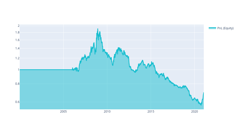
performance = stat.to_pandas()["equity"]
qngraph.make_plot_filled(performance.index, performance, name="PnL (Equity)", type="log")

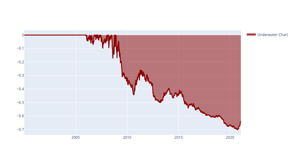
UWchart = stat.to_pandas()["underwater"]
qngraph.make_plot_filled(UWchart.index, UWchart, color="darkred", name="Underwater Chart", range_max=0)

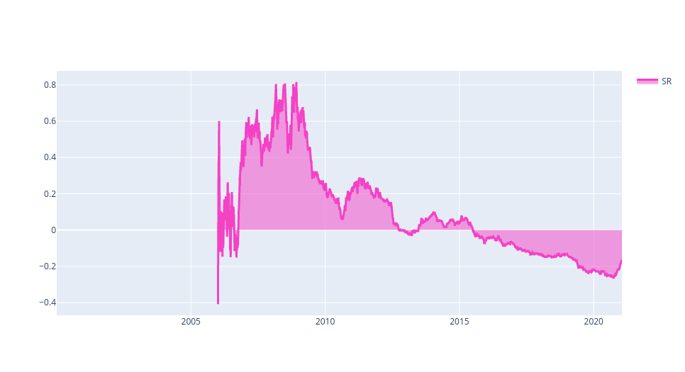
SRchart = stat.to_pandas()["sharpe_ratio"]
qngraph.make_plot_filled(SRchart.index, SRchart, color="#F442C5", name="SR")