Acess previous weights
-
or if not. Is there code available of the competition backtest, so I may figure out a way.
Thx -
@magenta-kabuto Hello. I didn't understand your question. If you need portfolio weights for the previous day, you can use
weights.shift(time=1)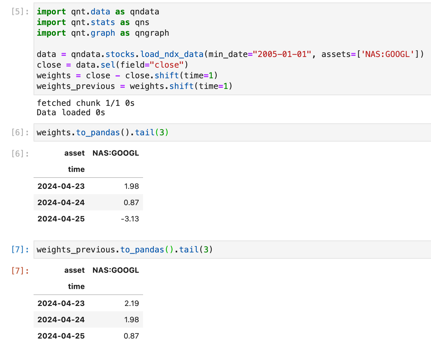
import qnt.data as qndata data = qndata.stocks.load_ndx_data(min_date="2005-01-01", assets=['NAS:GOOGL']) close = data.sel(field="close") weights = close - close.shift(time=1) weights_previous = weights.shift(time=1) -
Hi @vyacheslav_b , thx for your reply.
Sry I expressed myself badly. What I mean is that as I understand if I predict each time step, my for example machine learning model, will take a position in t (lets say 0.5). Now in t+1 when the notebook is run again for prediction that information is lost ,isnt it? So if I want to apply the lower slippage, how can I do that?
An example is the screenshot I posted above, which makes a one step prediction, by assigning a weight for selected assets on the latest index at time step t. No tomorrow in t+1 it will assign a new weight for the selcted assets without knowledge what was assigned in t with the knowledge in t, as in t+1 I could take the value of the prediction for (which is part of the batch) but will be different from the weights I assigned in t because of forward looking.
I hope I didnt overcomplicate in my expression.
Regards -
Hey @support,
can you maybe help?
Is there a way to download or access weights like its done for data? (which is updated for each time step)
Thank you.
Regards -
@magenta-kabuto Hi, I am not sure I understand you correctly, maybe you can use the stateful version of the backtester as we described here:
https://quantiacs.com/documentation/en/reference/evaluation.html#stateful-multi-pass-backtesting
which will preserve in memory previous state.
-
@support thx for your reply.
I also saw some discussion related to a similar topic in the general discussion.
I will try to explain what I mean, if it doesnt make sense just ignore it and if I get something wrong, pls let me know.
The point i am making is lets imagine the evaluation period starts on 01.06.2024 and my Deep Learning model meets the criteria for evaluation.
Now since 01.06.2024 is the first day, the model will predict for this day and assign the weights for assets traded on 01.06.2024, one day before, where it is trained.
Now to my understanding, the model is retrained everyday for the single-pass submission of the DL-Model, which therefore will have different weights (model weights, not allocation weights) for the next day training (01.06.2024) and will predict one step ahead, the allocations for 02.06.2024, and so on.
So my question is, that under this framework I do not have access to the previous weights, right ? (For 01.06.2024 model training, I do not know what allocation weights I assigned on 31.05.2024)(I dont know whether with the stateful model I can have access to lets say up to 60 days of previous allocations)
The weights assigned however, are saved somewhere with quantiacs ,as these allocation were made in the past but are not accessible to me ,lets say on 03.06.2024.
SO if I want to reduce slippage, so that I on 03.06.2024 want to change allocations only if the predictions are larger since the beginning of the evaluation, how can I do that.
I hope it makes sense what I am trying to say.
Regards -
Hi @support,
just wanted to thank for the suggestion of the stateful backtester, as this solves the issue.
I incorporated the DL model into the stateful backtester, which seems to work (backtesting right-now).
And the get_lower slippage function in the ML- templates is subject to forward looking, overfitting the holding period.
Regards -
@magenta-kabuto Hello. Use the following example.
Note that the backtest parameters are set for daily prediction of values.
The prediction function is designed to return a value for one day. Later, I will show how to create a single-pass version.import xarray as xr import qnt.data as qndata import qnt.backtester as qnbt import qnt.ta as qnta import qnt.stats as qns import qnt.graph as qngraph import qnt.output as qnout import numpy as np import pandas as pd import torch from torch import nn, optim import random asset_name_all = ['NAS:AAPL', 'NAS:GOOGL'] lookback_period = 155 train_period = 100 class LSTM(nn.Module): """ Class to define our LSTM network. """ def __init__(self, input_dim=3, hidden_layers=64): super(LSTM, self).__init__() self.hidden_layers = hidden_layers self.lstm1 = nn.LSTMCell(input_dim, self.hidden_layers) self.lstm2 = nn.LSTMCell(self.hidden_layers, self.hidden_layers) self.linear = nn.Linear(self.hidden_layers, 1) def forward(self, y): outputs = [] n_samples = y.size(0) h_t = torch.zeros(n_samples, self.hidden_layers, dtype=torch.float32) c_t = torch.zeros(n_samples, self.hidden_layers, dtype=torch.float32) h_t2 = torch.zeros(n_samples, self.hidden_layers, dtype=torch.float32) c_t2 = torch.zeros(n_samples, self.hidden_layers, dtype=torch.float32) for time_step in range(y.size(1)): x_t = y[:, time_step, :] # Ensure x_t is [batch, input_dim] h_t, c_t = self.lstm1(x_t, (h_t, c_t)) h_t2, c_t2 = self.lstm2(h_t, (h_t2, c_t2)) output = self.linear(h_t2) outputs.append(output.unsqueeze(1)) outputs = torch.cat(outputs, dim=1).squeeze(-1) return outputs def get_model(): def set_seed(seed_value=42): """Set seed for reproducibility.""" random.seed(seed_value) np.random.seed(seed_value) torch.manual_seed(seed_value) torch.cuda.manual_seed(seed_value) torch.cuda.manual_seed_all(seed_value) # if you are using multi-GPU. torch.backends.cudnn.deterministic = True torch.backends.cudnn.benchmark = False set_seed(42) model = LSTM(input_dim=3) return model def get_features(data): close_price = data.sel(field="close").ffill('time').bfill('time').fillna(1) open_price = data.sel(field="open").ffill('time').bfill('time').fillna(1) high_price = data.sel(field="high").ffill('time').bfill('time').fillna(1) log_close = np.log(close_price) log_open = np.log(open_price) features = xr.concat([log_close, log_open, high_price], "feature") return features def get_target_classes(data): price_current = data.sel(field='open') price_future = qnta.shift(price_current, -1) class_positive = 1 # prices goes up class_negative = 0 # price goes down target_price_up = xr.where(price_future > price_current, class_positive, class_negative) return target_price_up def load_data(period): return qndata.stocks.load_ndx_data(tail=period, assets=asset_name_all) def train_model(data): features_all = get_features(data) target_all = get_target_classes(data) models = dict() for asset_name in asset_name_all: model = get_model() target_cur = target_all.sel(asset=asset_name).dropna('time', 'any') features_cur = features_all.sel(asset=asset_name).dropna('time', 'any') target_for_learn_df, feature_for_learn_df = xr.align(target_cur, features_cur, join='inner') criterion = nn.MSELoss() optimiser = optim.LBFGS(model.parameters(), lr=0.08) epochs = 1 for i in range(epochs): def closure(): optimiser.zero_grad() feature_data = feature_for_learn_df.transpose('time', 'feature').values in_ = torch.tensor(feature_data, dtype=torch.float32).unsqueeze(0) out = model(in_) target = torch.zeros(1, len(target_for_learn_df.values)) target[0, :] = torch.tensor(np.array(target_for_learn_df.values)) loss = criterion(out, target) loss.backward() return loss optimiser.step(closure) models[asset_name] = model return models def predict(models, data, state): last_time = data.time.values[-1] data_last = data.sel(time=slice(last_time, None)) weights = xr.zeros_like(data_last.sel(field='close')) for asset_name in asset_name_all: features_all = get_features(data_last) features_cur = features_all.sel(asset=asset_name).dropna('time', 'any') if len(features_cur.time) < 1: continue feature_data = features_cur.transpose('time', 'feature').values in_ = torch.tensor(feature_data, dtype=torch.float32).unsqueeze(0) out = models[asset_name](in_) prediction = out.detach()[0] weights.loc[dict(asset=asset_name, time=features_cur.time.values)] = prediction weights = weights * data_last.sel(field="is_liquid") # state may be null, so define a default value if state is None: default = xr.zeros_like(data_last.sel(field='close')).isel(time=-1) state = { "previus_weights": default, } previus_weights = state['previus_weights'] # align the arrays to prevent problems in case the asset list changes previus_weights, weights = xr.align(previus_weights, weights, join='right') weights_avg = (previus_weights + weights) / 2 next_state = { "previus_weights": weights_avg.isel(time=-1), } # print(last_time) # print("previus_weights") # print(previus_weights) # print(weights) # print("weights_avg") # print(weights_avg.isel(time=-1)) return weights_avg, next_state weights = qnbt.backtest_ml( load_data=load_data, train=train_model, predict=predict, train_period=train_period, retrain_interval=360, retrain_interval_after_submit=1, predict_each_day=True, competition_type='stocks_nasdaq100', lookback_period=lookback_period, start_date='2006-01-01', build_plots=True )I recommend not using state at all, but rather using the approach I mentioned above.
Because it's faster.
If you need to use a single-pass version, it's better to load more data and calculate the weight values for previous days, then combine them. You will have calculated weights for the previous days. -
@vyacheslav_b Hi. I would like to ask how to switch from ml_backtest to single backtest to submit? And will this move lead to forward looking risks?
If so, is there no way to satisfy submission without exceeding time while eliminating forward looking? Looking forward to your answers and support. Thank you.
-
Hi @vyacheslav_b ,
thank you very much for the solution.
I did not know that the ML_backtester is capable of handling two outputs (weights and state) but I will from now on use it.
Regards -
@vyacheslav_b the problem with not using states as I understand is the following: lets say the model estimated in t (single pass) gives an estimate for NAS:AAPL = 0.04 (weight allocation). So thats the position assigned to the stock in t for t+1.
In t+1 the model is reestimated but with the information of NAS:AAPL in t and assigns weights 0.03 for t+1 and 0.035 for t+2 in t+1. When I do not use states, and apply get_lower_slippage function , I will have weight allocation 0.035 for t+2 in t+1 whereas with the states I will have 0.04 for t+2 in t+1 and I will not have impact of the transaction costs.
Thank you.
Regards -
@vyacheslav_b I tried your way but when prechecking there was an error: some dates are missed in the portfolio_history and the sharpness was very low.
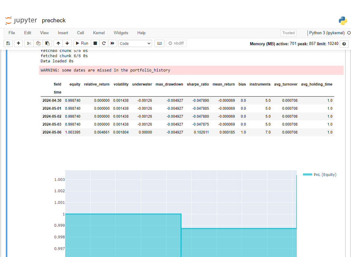
I went to precheck result html file and this is the error result and sharpe is nan
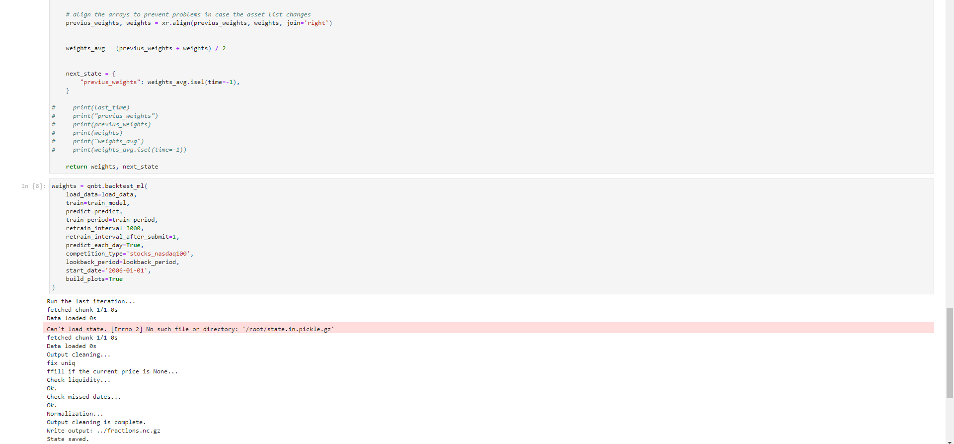
We look forward to receiving your support. Thank you
@support @Vyacheslav_B -
@machesterdragon Hello.
If you use a state and a function that returns the prediction for one day, you will not get correct results with precheck.
Theoretically, you can specify the number of partitions as all available days. or you can return all predictions
I have not checked how the precheck works.
If it works in parallel, you will not see the correct result even more so.
State in strategy limits you. I recommend not using it.
Here is an example of a version for one pass; I couldn't test it because my submission did not calculate even one day.
init.ipynb
! pip install torch==2.2.1strategy.ipynb
import gzip
import pickle

from qnt.data import get_env
from qnt.log import log_err, log_info


def state_write(state, path=None):
    if path is None:
        path = get_env("OUT_STATE_PATH", "state.out.pickle.gz")
    try:
        with gzip.open(path, 'wb') as gz:
            pickle.dump(state, gz)
        log_info("State saved: " + str(state))
    except Exception as e:
        log_err(f"Error saving state: {e}")


def state_read(path=None):
    if path is None:
        path = get_env("OUT_STATE_PATH", "state.out.pickle.gz")
    try:
        with gzip.open(path, 'rb') as gz:
            state = pickle.load(gz)
        log_info("State loaded.")
        return state
    except Exception as e:
        log_err(f"Can't load state: {e}")
        return None


state = state_read()
print(state)


# separate cell

def print_stats(data, weights):
    stats = qns.calc_stat(data, weights)
    display(stats.to_pandas().tail())
    performance = stats.to_pandas()["equity"]
    qngraph.make_plot_filled(performance.index, performance, name="PnL (Equity)", type="log")


data_train = load_data(train_period)
models = train_model(data_train)

data_predict = load_data(lookback_period)

last_time = data_predict.time.values[-1]

if last_time < np.datetime64('2006-01-02'):
    print("The first state should be None")
    state_write(None)
    state = state_read()
    print(state)

weights_predict, state_new = predict(models, data_predict, state)

print_stats(data_predict, weights_predict)
state_write(state_new)
print(state_new)
qnout.write(weights_predict)  # To participate in the competition, save this code in a separate cell.
But I hope it will work correctly.
Do not expect any responses from me during this week.
-
@vyacheslav_b said in Acess previous weights:
If you use a state and a function that returns the prediction for one day, you will not get correct results with precheck.
Theoretically, you can specify the number of partitions as all available days. or you can return all predictions
I have not checked how the precheck works.
If it works in parallel, you will not see the correct result even more so.
State in strategy limits you. I recommend not using it.Thank you so much @Vyacheslav_B.
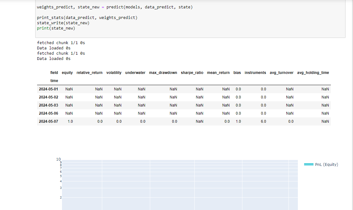
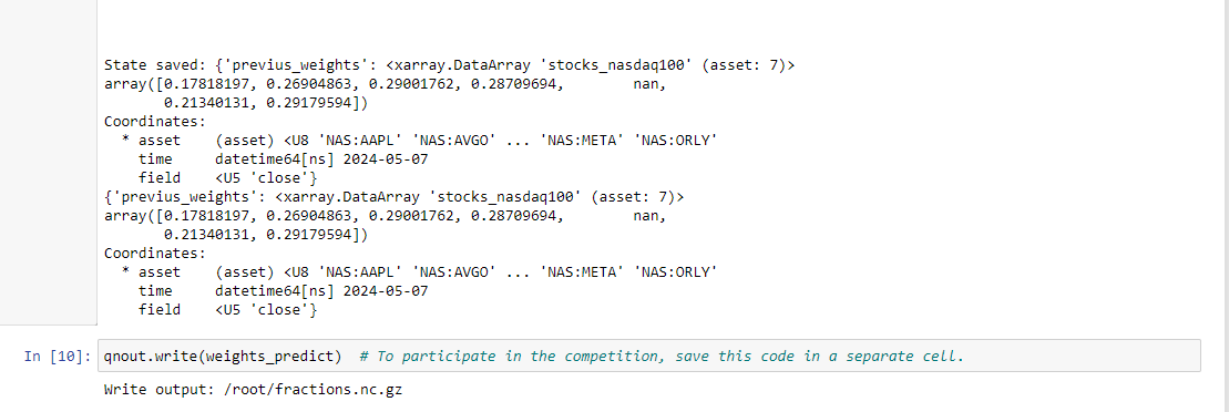
I just tried applying the single pass you suggested but the results were nan. Looking forward to your help when you have time. thank you very much
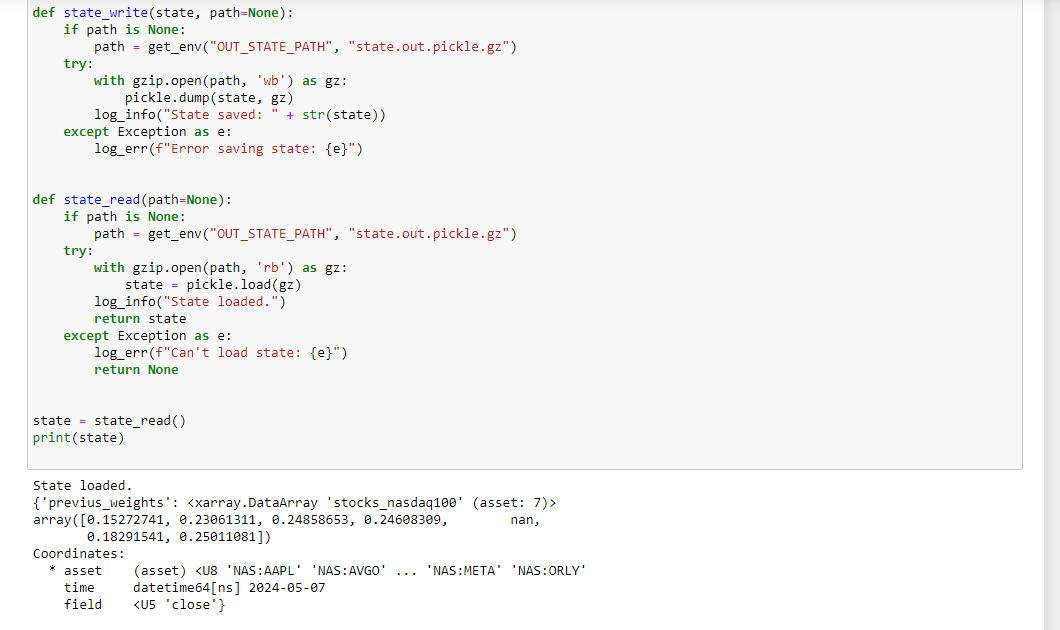
-
@machesterdragon
That's how it should be. This code is needed so that submissions are processed faster when sent to the contest. The backtest system will calculate the weights for each day. The function I provided calculates weights for only one day. -
@vyacheslav_b Hello, I was trying the code you gave and realized that using state for train ml_backtest only works when the get feature function is a feature like ohlc or log of ohlc (open, high, low, close).
I added some other features (eg: trend = qnta.roc(qnta.lwma(data.sel(field='close'), 40), 1),...) and noticed that after passing ml_backtest, every The indexes are all nan. Looking forward to your help. Thank you.
-
@illustrious-felice Hello.
Show me an example of the code.
I don't quite understand what you are trying to do.
Maybe you just don't have enough data in the functions to get the value.
Please note that in the lines I intentionally reduce the data size to 1 day to predict only the last day.
last_time = data.time.values[-1]
data_last = data.sel(time=slice(last_time, None))
Calculate your indicators before this code, and then slice the values.
-
@vyacheslav_b Thank you for your response
Here is the code I used from your example. I added some other features (eg: trend = qnta.roc(qnta.lwma(data.sel(field='close'), 40), 1),...) and noticed that after passing ml_backtest, every indexes are all nan. Pnl is a straight line. I have tried changing many other features but the result is still the same, all indicators are nanimport xarray as xr import qnt.data as qndata import qnt.backtester as qnbt import qnt.ta as qnta import qnt.stats as qns import qnt.graph as qngraph import qnt.output as qnout import numpy as np import pandas as pd import torch from torch import nn, optim import random asset_name_all = ['NAS:AAPL', 'NAS:GOOGL'] lookback_period = 155 train_period = 100 class LSTM(nn.Module): """ Class to define our LSTM network. """ def __init__(self, input_dim=3, hidden_layers=64): super(LSTM, self).__init__() self.hidden_layers = hidden_layers self.lstm1 = nn.LSTMCell(input_dim, self.hidden_layers) self.lstm2 = nn.LSTMCell(self.hidden_layers, self.hidden_layers) self.linear = nn.Linear(self.hidden_layers, 1) def forward(self, y): outputs = [] n_samples = y.size(0) h_t = torch.zeros(n_samples, self.hidden_layers, dtype=torch.float32) c_t = torch.zeros(n_samples, self.hidden_layers, dtype=torch.float32) h_t2 = torch.zeros(n_samples, self.hidden_layers, dtype=torch.float32) c_t2 = torch.zeros(n_samples, self.hidden_layers, dtype=torch.float32) for time_step in range(y.size(1)): x_t = y[:, time_step, :] # Ensure x_t is [batch, input_dim] h_t, c_t = self.lstm1(x_t, (h_t, c_t)) h_t2, c_t2 = self.lstm2(h_t, (h_t2, c_t2)) output = self.linear(h_t2) outputs.append(output.unsqueeze(1)) outputs = torch.cat(outputs, dim=1).squeeze(-1) return outputs def get_model(): def set_seed(seed_value=42): """Set seed for reproducibility.""" random.seed(seed_value) np.random.seed(seed_value) torch.manual_seed(seed_value) torch.cuda.manual_seed(seed_value) torch.cuda.manual_seed_all(seed_value) # if you are using multi-GPU. torch.backends.cudnn.deterministic = True torch.backends.cudnn.benchmark = False set_seed(42) model = LSTM(input_dim=3) return model def get_features(data): close_price = data.sel(field="close").ffill('time').bfill('time').fillna(1) open_price = data.sel(field="open").ffill('time').bfill('time').fillna(1) high_price = data.sel(field="high").ffill('time').bfill('time').fillna(1) log_close = np.log(close_price) log_open = np.log(open_price) trend = qnta.roc(qnta.lwma(close_price ), 40), 1) features = xr.concat([log_close, log_open, high_price, trend], "feature") return features def get_target_classes(data): price_current = data.sel(field='open') price_future = qnta.shift(price_current, -1) class_positive = 1 # prices goes up class_negative = 0 # price goes down target_price_up = xr.where(price_future > price_current, class_positive, class_negative) return target_price_up def load_data(period): return qndata.stocks.load_ndx_data(tail=period, assets=asset_name_all) def train_model(data): features_all = get_features(data) target_all = get_target_classes(data) models = dict() for asset_name in asset_name_all: model = get_model() target_cur = target_all.sel(asset=asset_name).dropna('time', 'any') features_cur = features_all.sel(asset=asset_name).dropna('time', 'any') target_for_learn_df, feature_for_learn_df = xr.align(target_cur, features_cur, join='inner') criterion = nn.MSELoss() optimiser = optim.LBFGS(model.parameters(), lr=0.08) epochs = 1 for i in range(epochs): def closure(): optimiser.zero_grad() feature_data = feature_for_learn_df.transpose('time', 'feature').values in_ = torch.tensor(feature_data, dtype=torch.float32).unsqueeze(0) out = model(in_) target = torch.zeros(1, len(target_for_learn_df.values)) target[0, :] = torch.tensor(np.array(target_for_learn_df.values)) loss = criterion(out, target) loss.backward() return loss optimiser.step(closure) models[asset_name] = model return models def predict(models, data, state): last_time = data.time.values[-1] data_last = data.sel(time=slice(last_time, None)) weights = xr.zeros_like(data_last.sel(field='close')) for asset_name in asset_name_all: features_all = get_features(data_last) features_cur = features_all.sel(asset=asset_name).dropna('time', 'any') if len(features_cur.time) < 1: continue feature_data = features_cur.transpose('time', 'feature').values in_ = torch.tensor(feature_data, dtype=torch.float32).unsqueeze(0) out = models[asset_name](in_) prediction = out.detach()[0] weights.loc[dict(asset=asset_name, time=features_cur.time.values)] = prediction weights = weights * data_last.sel(field="is_liquid") # state may be null, so define a default value if state is None: default = xr.zeros_like(data_last.sel(field='close')).isel(time=-1) state = { "previus_weights": default, } previus_weights = state['previus_weights'] # align the arrays to prevent problems in case the asset list changes previus_weights, weights = xr.align(previus_weights, weights, join='right') weights_avg = (previus_weights + weights) / 2 next_state = { "previus_weights": weights_avg.isel(time=-1), } # print(last_time) # print("previus_weights") # print(previus_weights) # print(weights) # print("weights_avg") # print(weights_avg.isel(time=-1)) return weights_avg, next_state weights = qnbt.backtest_ml( load_data=load_data, train=train_model, predict=predict, train_period=train_period, retrain_interval=360, retrain_interval_after_submit=1, predict_each_day=True, competition_type='stocks_nasdaq100', lookback_period=lookback_period, start_date='2006-01-01', build_plots=True )


-
hello again to all,
I hope everyone is fine.
I again came across a question, which should have occurred to me earlier, namely when we use a stateful machine learning strategy for submission, how can we pass on the states without using the ml_backtester, assuming the notebook is rerun at each point in time.
Thank you.
Regards -
https://github.com/quantiacs/strategy-ml_lstm_state/blob/master/strategy.ipynb
This repository provides an example of using state, calculating complex indicators, dynamically selecting stocks for trading, and implementing basic risk management measures, such as normalizing and reducing large positions. It also includes recommendations for submitting strategies to the competition.