Data loading
This section contains the detailed API reference documentation. It is intended for users who are already familiar with the Quantiacs platform. First-time users can start at the Quick start page.
Inspecting the list of stocks
The available stocks in the NASDAQ100 index can be inspected using the following function:
Function
import qnt.data as qndata
qndata.stocks.load_ndx_list(min_date = None, max_date = None, tail = 365 * 4)
Parameters
| Parameter | Explanation |
|---|---|
| min_date | filters the list from specific date (string, ‘yyyy-mm-dd’ format). Default None value uses max_date-tail. |
| max_date | last date of data. Default None value is current day. |
| tail | calendar days, min_date = max_date - tail. Default value is 6 years, 365 * 4. |
Output
The output is a list of dictionaries with info on name, sector, symbol, sector and more of all available stocks in the specified time frame:
[{'name': 'American Airlines Group',
  'sector': 'Consumer Goods',
  'symbol': 'AAL',
  'exchange': 'NAS',
  'id': 'NAS:AAL',
  'FIGI': 'tts-67645939'},
 {'name': 'Apple',
  'sector': 'IT/Telecommunications',
  'symbol': 'AAPL',
  'exchange': 'NAS',
  'id': 'NAS:AAPL',
  'FIGI': 'tts-831814'},
 {'name': 'Airbnb Inc',
  'sector': None,
  'symbol': 'ABNB',
  'exchange': 'NAS',
  'id': 'NAS:ABNB',
  'FIGI': 'tts-207966789'},
  ...
  {'name': 'Zoom Video Communications',
  'sector': None,
  'symbol': 'ZM',
  'exchange': 'NAS',
  'id': 'NAS:ZM',
  'FIGI': 'tts-163839424'},
 {'name': 'Zscaler',
  'sector': None,
  'symbol': 'ZS',
  'exchange': 'NAS',
  'id': 'NAS:ZS',
  'FIGI': 'tts-137190768'}]
Loading stocks data
Stocks data can be loaded using:
Function
import qnt.data as qndata
qndata.stocks.load_ndx_data(assets = None, min_date = None, max_date = None, dims = ('time', 'field', 'asset')),
    forward_order = True, tail = 365 * 6)
Parameters
| Parameter | Explanation |
|---|---|
| assets | list of ticker names to load, example: ["NAS:AAPL", "NAS:ABNB"]. Default None value loads all assets. |
| min_date | first date in data, example "2006-01-01". Default None value uses max_date-tail. |
| max_date | last date of data. Default None value is current day. |
| dims | tuple with "time","field", "asset" attributes in the specified order. |
| forward_order | boolean, default True value orders date in ascending order. |
| tail | calendar days, min_date = max_date - tail. Default value is 6 years, 365 * 6. |
Output
The output is an xarray.DataArray with historical data for the selected assets. Coordinates are:
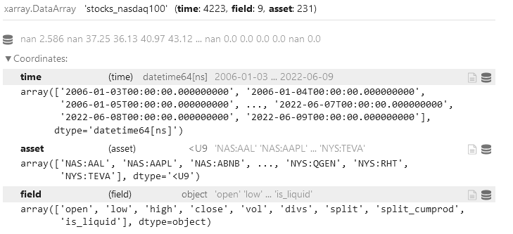
Example
One can load market data for Apple and Amazon stock for the past 10 years as follows:
import qnt.data as qndata
data = qndata.stocks.load_ndx_data(assets= ['NAS:AAPL', 'NAS:AMZN'], tail=365*10)
Specific fields can be extracted using:
open  = data.sel(field='open')
close = data.sel(field='close')
high  = data.sel(field='high')
low   = data.sel(field='low')

volume_day = data.sel(field='vol')
dividends = data.sel(field='divs')
where:
| Data field | Description |
|---|---|
| open | Opening daily price. |
| close | Closing daily price. |
| high | Highest daily price. |
| low | Lowest daily price. |
| vol | Daily trading volume(number of shares). |
| divs | Dividend payment. |
Data can be nicely displayed using:
open.to_pandas().head()
| asset time |
NAS:AAPL |
NAS:AMZN |
|---|---|---|
| 2012-06-25 | 20.6179 | 11.0150 |
| 2012-06-26 | 20.4046 | 11.0725 |
| 2012-06-27 | 20.5357 | 11.2505 |
| 2012-06-28 | 20.4168 | 11.1960 |
| 2012-06-29 | 20.6429 | 11.2350 |
Inspecting the list of futures
The available futures financial instruments can be inspected using the following function:
Function
import qnt.data as qndata
qndata.futures.load_list()
Output
The output is a list of dictionaries with info on ticker symbols and assets:
[{'id': 'F_AE',
  'name': 'AEX Index',
  'sector': 'Index',
  'point_value': 'EUR 200'},
 {'id': 'F_AH',
  'name': 'Bloomberg Commodity',
  'sector': 'Index',
  'point_value': '$250'},
 {'id': 'F_AX',
  'name': 'DAX Index',
  'sector': 'Index',
  'point_value': 'EUR 25'},
 {'id': 'F_BC',
  'name': 'Crude Oil Brent',
  'sector': 'Energy',
  'point_value': '$1,000'},
 {'id': 'F_BG',
  'name': 'ICE Gas Oil LS',
  'sector': 'Energy',
  'point_value': '$100'},
 {'id': 'F_C',
  'name': 'Corn',
  'sector': 'Agriculture',
  'point_value': 'EUR 50'},
 {'id': 'F_CA', 'name': 'CAC 40', 'sector': 'Index', 'point_value': 'EUR 10'},
 {'id': 'F_CC',
  'name': 'Cocoa',
  'sector': 'Agriculture',
  'point_value': '$10'},
 {'id': 'F_CF',
  'name': 'Eurex Conf Long-Term',
  'sector': 'Bond',
  'point_value': 'CHF 1,000'},
 {'id': 'F_CT',
  'name': 'Cotton #2',
  'sector': 'Agriculture',
  'point_value': '$500'},
 {'id': 'F_DE',
  'name': 'MSCI EMI Index',
  'sector': 'Index',
  'point_value': '$50'},
 {'id': 'F_DM',
  'name': 'MDAX Index',
  'sector': 'Index',
  'point_value': 'EUR 5'},
 {'id': 'F_DT',
  'name': 'Euro Bund',
  'sector': 'Bond',
  'point_value': 'EUR 1,000'},
 {'id': 'F_DX',
  'name': 'U.S. Dollar Index',
  'sector': 'Currency',
  'point_value': '$1,000'},
 {'id': 'F_EB',
  'name': 'Eurex 3Month EuriBor',
  'sector': 'InterestRate',
  'point_value': 'EUR 2,500'},
 {'id': 'F_ED',
  'name': 'LIFFE EuroDollar',
  'sector': 'InterestRate',
  'point_value': '$2,500'},
 {'id': 'F_F',
  'name': '3-Month Euroswiss',
  'sector': 'InterestRate',
  'point_value': 'CHF 2,500'},
 {'id': 'F_FB',
  'name': 'Stoxx Banks 600',
  'sector': 'Index',
  'point_value': 'EUR 50'},
 {'id': 'F_FP',
  'name': 'OMX Helsinki 25',
  'sector': 'Index',
  'point_value': 'EUR 10'},
 {'id': 'F_FY',
  'name': 'Stoxx Europe 600',
  'sector': 'Index',
  'point_value': 'EUR 50'},
 {'id': 'F_GC',
  'name': 'ICE Gold 100-oz',
  'sector': 'Metal',
  'point_value': '$100'},
 {'id': 'F_GS',
  'name': '10-Year Long Gilt',
  'sector': 'Bond',
  'point_value': 'GBP 1,000'},
 {'id': 'F_GX',
  'name': 'Euro Buxl',
  'sector': 'Bond',
  'point_value': 'EUR 1,000'},
 {'id': 'F_HG',
  'name': 'HKFE Copper CNH',
  'sector': 'Metal',
  'point_value': 'RMB 5'},
 {'id': 'F_HO',
  'name': 'ICE Heating Oil',
  'sector': 'Energy',
  'point_value': '$42,000'},
 {'id': 'F_KC',
  'name': 'Coffee',
  'sector': 'Agriculture',
  'point_value': '$375'},
 {'id': 'F_LX',
  'name': 'FTSE 100',
  'sector': 'Index',
  'point_value': 'GBP 10'},
 {'id': 'F_NG',
  'name': 'ICE UK Natural Gas',
  'sector': 'Energy',
  'point_value': 'GBP 1,000'},
 {'id': 'F_NH',
  'name': 'SGX CNX Nifty Index',
  'sector': 'Index',
  'point_value': '$20'},
 {'id': 'F_OJ',
  'name': 'Orange Juice',
  'sector': 'Agriculture',
  'point_value': '$150'},
 {'id': 'F_RB',
  'name': 'Tocom Gasoline',
  'sector': 'Energy',
  'point_value': 'JPY 50'},
 {'id': 'F_RU',
  'name': 'Russell 2000 E-Mini',
  'sector': 'Index',
  'point_value': '$50'},
 {'id': 'F_SB',
  'name': 'Sugar #11',
  'sector': 'Agriculture',
  'point_value': '$1,120'},
 {'id': 'F_SI',
  'name': 'ICE Silver 5000-oz',
  'sector': 'Metal',
  'point_value': '$5,000'},
 {'id': 'F_SS',
  'name': '3-Month Sterling',
  'sector': 'InterestRate',
  'point_value': 'GBP 1,250'},
 {'id': 'F_SX',
  'name': 'Swiss Market Index',
  'sector': 'Index',
  'point_value': 'CHF 10'},
 {'id': 'F_UB',
  'name': 'Euro Bobl',
  'sector': 'Bond',
  'point_value': 'EUR 1,000'},
 {'id': 'F_UZ',
  'name': 'Euro Schatz',
  'sector': 'Bond',
  'point_value': 'EUR 1,000'},
 {'id': 'F_VX',
  'name': 'S&P 500 VIX',
  'sector': 'Index',
  'point_value': '$1,000'},
 {'id': 'F_W',
  'name': 'Milling Wheat',
  'sector': 'Agriculture',
  'point_value': 'EUR 50'},
 {'id': 'F_XX',
  'name': 'Stoxx 50',
  'sector': 'Index',
  'point_value': 'EUR 10'},
 {'id': 'F_AD',
  'name': 'Australian Dollar',
  'sector': 'Currency',
  'point_value': '1'},
 {'id': 'F_BP',
  'name': 'British Pound',
  'sector': 'Currency',
  'point_value': '1'},
 {'id': 'F_CD',
  'name': 'Canadian Dollar',
  'sector': 'Currency',
  'point_value': '1'},
 {'id': 'F_EC', 'name': 'Euro', 'sector': 'Currency', 'point_value': '1'},
 {'id': 'F_JY',
  'name': 'Japanese Yen',
  'sector': 'Currency',
  'point_value': '1'},
 {'id': 'F_MP',
  'name': 'Mexican Peso',
  'sector': 'Currency',
  'point_value': '1'},
 {'id': 'F_SF',
  'name': 'Swiss Frank',
  'sector': 'Currency',
  'point_value': '1'},
 {'id': 'F_LR',
  'name': 'Brazilian Real',
  'sector': 'Currency',
  'point_value': '1'},
 {'id': 'F_ND',
  'name': 'New Zealand Dollar',
  'sector': 'Currency',
  'point_value': '1'},
 {'id': 'F_QT',
  'name': 'Chinese Yuan',
  'sector': 'Currency',
  'point_value': '1'},
 {'id': 'F_RF',
  'name': 'Euro / Swiss Franc',
  'sector': 'Currency',
  'point_value': '1'},
 {'id': 'F_RP',
  'name': 'Euro / British Pound',
  'sector': 'Currency',
  'point_value': '1'},
 {'id': 'F_RR',
  'name': 'Russian Ruble',
  'sector': 'Currency',
  'point_value': '1'},
 {'id': 'F_RY',
  'name': 'Euro / Japanese Yen',
  'sector': 'Currency',
  'point_value': '1'},
 {'id': 'F_TR',
  'name': 'South African Rand',
  'sector': 'Currency',
  'point_value': '1'},
 {'id': 'F_BO',
  'name': 'WisdomTree Soybean Oil',
  'sector': 'Agriculture',
  'point_value': '1'},
 {'id': 'F_CL',
  'name': 'United States Oil Fund',
  'sector': 'Energy',
  'point_value': '1'},
 {'id': 'F_FV',
  'name': 'BTC iShares 3-7 Year Treasury Bond ETF',
  'sector': 'Bond',
  'point_value': '1'},
 {'id': 'F_MD',
  'name': 'iShares Core S&P Mid-Cap ETF',
  'sector': 'Index',
  'point_value': '1'},
 {'id': 'F_NQ',
  'name': 'Invesco QQQ Trust Series 1',
  'sector': 'Index',
  'point_value': '1'},
 {'id': 'F_PA',
  'name': 'Aberdeen Standard Physical Palladium Shares ETF',
  'sector': 'Metal',
  'point_value': '1'},
 {'id': 'F_PL',
  'name': 'Aberdeen Standard Physical Platinum Shares ETF',
  'sector': 'Metal',
  'point_value': '1'},
 {'id': 'F_TU',
  'name': 'BTC iShares 1-3 Year Treasury Bond ETF',
  'sector': 'Bond',
  'point_value': '1'},
 {'id': 'F_TY',
  'name': 'BTC iShares 7-10 Year Treasury Bond ETF',
  'sector': 'Bond',
  'point_value': '1'},
 {'id': 'F_US',
  'name': 'BTC iShares U.S. Treasury Bond ETF',
  'sector': 'Bond',
  'point_value': '1'},
 {'id': 'F_YM',
  'name': 'SPDR Dow Jones Industrial Average ETF',
  'sector': 'Index',
  'point_value': '1'},
 {'id': 'F_S',
  'name': 'WisdomTree Soybeans',
  'sector': 'Agriculture',
  'point_value': '1'},
 {'id': 'F_NY',
  'name': 'iShares MSCI Japan ETF',
  'sector': 'Index',
  'point_value': '1'},
 {'id': 'F_AG',
  'name': 'Invesco DB Agriculture Fund',
  'sector': 'Agriculture',
  'point_value': '1'},
 {'id': 'F_ES',
  'name': 'S&P 500 ETF TRUST ETF',
  'sector': 'Index',
  'point_value': '1'}]
Loading futures data
Futures data can be loaded using:
Function
import qnt.data as qndata
qndata.futures.load_data(assets = None, min_date = None, max_date = None, dims = ("field", "time", "asset"),
    forward_order = True, tail = 365 * 6, offset = 0)
Parameters
| Parameter | Explanation |
|---|---|
| assets | list of ticker names to load, example: ["F_AD", "F_BO"]. Default None value loads all assets. |
| min_date | first date in data, example "2006-01-01". Default None value uses max_date-tail. |
| max_date | last date of data. Default None value is current day. |
| dims | tuple with "field", "time", "asset" attributes in the specified order. |
| forward_order | boolean, default True value orders date in ascending order. |
| tail | calendar days, min_date = max_date - tail. Default value is 6 years, 365 * 6. |
| offset | switch for selecting maturity: 0/1/2, front/next-to-front/next-to-next-to-front. |
Output
The output is an xarray.DataArray with historical data for the selected assets. Coordinates are:
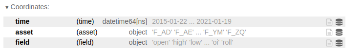
Example
One can load market data for the Australian Dollar/US Dollar rate and Soybean Oil for the past 15 years as follows:
import qnt.data as qndata
data = qndata.futures.load_data(assets= ['F_AD', 'F_BO'], tail=365*15)
Specific fields can be extracted using:
open  = data.sel(field='open')
close = data.sel(field='close')
high  = data.sel(field='high')
low   = data.sel(field='low')

volume_day    = data.sel(field='vol')
open_interest = data.sel(field='oi')

contracts_roll_over = data.sel(field='roll')
where:
| Data field | Description |
|---|---|
| open | Opening daily price. |
| close | Closing daily price. |
| high | Highest daily price. |
| low | Lowest daily price. |
| vol | Daily trading volume (number of contracts). |
| oi | Total number of outstanding contracts. |
| roll | Futures contract rollover information. |
Data can be nicely displayed using:
open.to_pandas().head()
| asset time |
F_AD |
F_BO |
|---|---|---|
| 2016-01-24 | 0.7527 | 21.55 |
| 2016-01-25 | 0.7501 | 21.50 |
| 2016-01-26 | 0.7523 | 21.52 |
| 2016-01-27 | 0.7502 | 21.57 |
| 2016-01-30 | 0.7485 | 22.11 |
Loading Bitcoin futures data
Bitcoin Futures data can be loaded using:
Function
import qnt.data as qndata
qndata.cryptofutures.load_data(assets = None, min_date = None, max_date = None, dims = ('field', 'time', 'asset'),
    forward_order = True, tail = 365 * 6)
Parameters
| Parameter | Explanation |
|---|---|
| assets | Default None value loads the Bitcoin Futures. |
| min_date | first date in data, example "2016-01-01". Default None value uses max_date-tail. |
| max_date | last date of data. Default None value is current day. |
| dims | tuple with "field", "time", "asset" attributes in the specified order. |
| forward_order | boolean, default True value orders date in ascending order. |
| tail | calendar days, min_date = max_date - tail. Default value is 6 years, 365 * 6. |
Output
The output is an xarray.DataArray with historical data for the selected assets. Coordinates are:
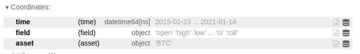
Example
One can load market data for the BTC Futures for the past 7 years as follows:
import qnt.data as qndata
data = qndata.cryptofutures.load_data(tail=365*7)
Specific fields can be extracted using:
open  = data.sel(field='open')
close = data.sel(field='close')
high  = data.sel(field='high')
low   = data.sel(field='low')

volume_day    = data.sel(field='vol')
open_interest = data.sel(field='oi')

contracts_roll_over = data.sel(field='roll')
where:
| Data field | Description |
|---|---|
| open | Opening daily price. |
| close | Closing daily price. |
| high | Highest daily price. |
| low | Lowest daily price. |
| vol | Daily trading volume (number of contracts). |
| oi | Total number of outstanding contracts. |
| roll | Futures contract rollover information. |
Data can be nicely displayed using:
open.to_pandas().head()
| asset time |
BTC |
|---|---|
| 2014-01-23 | 850.0 |
| 2014-01-24 | 847.0 |
| 2014-01-27 | 852.0 |
| 2014-01-28 | 800.0 |
| 2014-01-29 | 826.0 |
Because of the short history of the Bitcoin Futures, we have patched its history with the spot Bitcoin one to go back in history.
Loading cryptocurrency daily data
This data can be loaded using:
Function
import qnt.data as qndata
qndata.cryptodaily.load_data(assets = None, min_date = None, max_date = None, dims = ('field', 'time', 'asset'),
    forward_order = True, tail = 365 * 6)
Parameters
| Parameter | Explanation |
|---|---|
| assets | list of ticker names to load, example: ["BTC", "ETH"]. Default None value loads all currencies. |
| min_date | first date in data, example "2014-01-01". Default None value uses max_date-tail. |
| max_date | last date of data. Default None value is current day. |
| dims | tuple with "field", "time", "asset" attributes in the specified order. |
| forward_order | boolean, default True value orders date in ascending order. |
| tail | calendar days, min_date = max_date - tail. Default value is 6 years, 365 * 6. |
Output
The output is an xarray.DataArray with historical data for the selected currencies. Coordinates are:
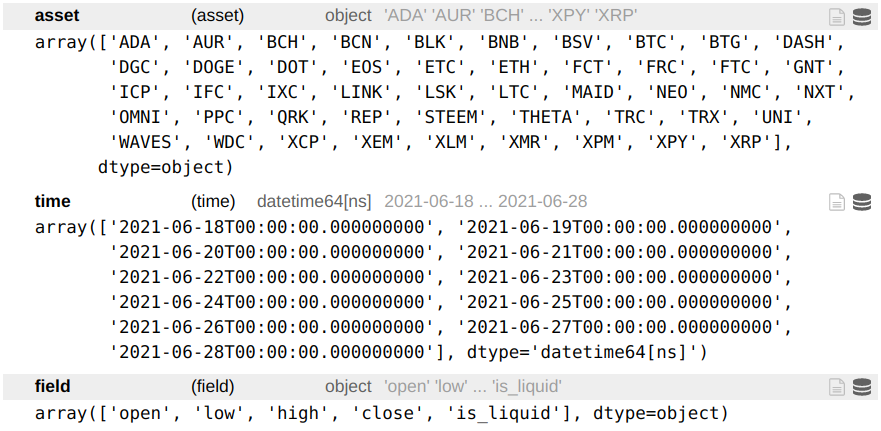
Example
One can load market data for BTC and ETH for the past 5 years as follows:
import qnt.data as qndata
data = qndata.cryptodaily.load_data(assets= ['BTC', 'ETH'], tail=365*5)
Specific fields can be extracted using:
open  = data.sel(field='open')
close = data.sel(field='close')
high  = data.sel(field='high')
low   = data.sel(field='low')

is_liquid = data.sel(field='is_liquid')
where:
| Data field | Description |
|---|---|
| open | Opening daily price. |
| close | Closing daily price. |
| high | Highest daily price. |
| low | Lowest daily price. |
| is_liquid | Is this cryptocurrency liquid? |
The system allows trading only liquid currencies, so you need to multiply the weights by is_liquid in your code.
weights = weights * is_liquid
Data can be nicely displayed using:
open.to_pandas().head()
| time | BTC | ETH |
|---|---|---|
| 2016-07-03 00:00:00 | 702.48 | 12.04 |
| 2016-07-04 00:00:00 | 659.77 | 11.67 |
| 2016-07-05 00:00:00 | 678.74 | 11.39 |
| 2016-07-06 00:00:00 | 669.09 | 10.5 |
| 2016-07-07 00:00:00 | 674.7 | 10.61 |
Loading cryptocurrency hourly data
Cryptocurrency data for:
Bitcoin (BTC);
Bitcoin Cash (BCH);
EOS;
Ethereum (ETH);
Litecoin (LTC);
Ripple (XRP);
Tether (USDT);
can be loaded using:
Function
import qnt.data as qndata
qndata.crypto.load_data(assets = None, min_date = None, max_date = None, dims = ('field', 'time', 'asset'),
    forward_order = True, tail = 365 * 6)
Parameters
| Parameter | Explanation |
|---|---|
| assets | list of assets, example ["ETH"]. Default None value loads all assets. |
| min_date | first date in data, example "2016-01-01". Default None value uses max_date-tail. |
| max_date | last date of data. Default None value is current day. |
| dims | tuple with "field", "time", "asset" attributes in the specified order. |
| forward_order | boolean, default True value orders date in ascending order. |
| tail | calendar days, min_date = max_date - tail. Default value is 6 years, 365 * 6. |
Output
The output is an xarray.DataArray with hourly historical data for the selected assets. Coordinates are:
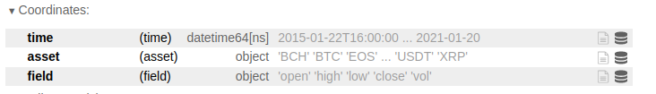
Example
One can load market data for Ethereum for the past 5 years as follows:
import qnt.data as qndata
data = qndata.crypto.load_data(assets= ['ETH'], tail=365*5)
Specific fields can be extracted using:
open  = data.sel(field='open')
close = data.sel(field='close')
high  = data.sel(field='high')
low   = data.sel(field='low')

volume    = data.sel(field='vol')
where:
| Data field | Description |
|---|---|
| open | First price in a given hour. |
| close | Last price in a given hour. |
| high | Highest price in a given hour. |
| low | Lowest price in a given hour. |
| vol | Hourly trading volume. |
Data can be nicely displayed using:
open.to_pandas().head()
| asset time |
ETH |
|---|---|
| 2016-03-09 16:00:00 | 10.297 |
| 2016-03-09 17:00:00 | 11.197 |
| 2016-03-09 18:00:00 | 11.097 |
| 2016-03-09 20:00:00 | 11.195 |
| 2016-03-09 21:00:00 | 10.870 |