Algorithm quality
After developing an algorithm, you can evaluate its performance using statistical indicators like the equity chart.
There are two main ways to evaluate your algorithm:
Single-Pass Backtesting
With single-pass backtesting you give a set of allocation weights (fractions of capital to be invested) for all assets over the entire backtesting period.
This approach evaluates your strategy quickly, but it cannot check whether your algorithm uses future data when determining allocation weights.
Let us consider a simple long-only strategy on the S&P500 Index Futures: we go long once the Simple Moving Average (qnta.sma) of the close price over the last 20 trading days is larger than the Simple Moving Average of the close price over the last 150 trading days.
import xarray as xr
import qnt.ta as qnta
import qnt.data as qndata
import qnt.output as qnout
data = qndata.futures_load_data(tail=365 * 15, assets= ['F_ES'])
close = data.sel(field='close')
sma150 = qnta.sma(close, 150)
sma20 = qnta.sma(close, 20)
weights = xr.where(sma150 < sma20, 1, 0)
weights = weights / abs(weights).sum('asset')
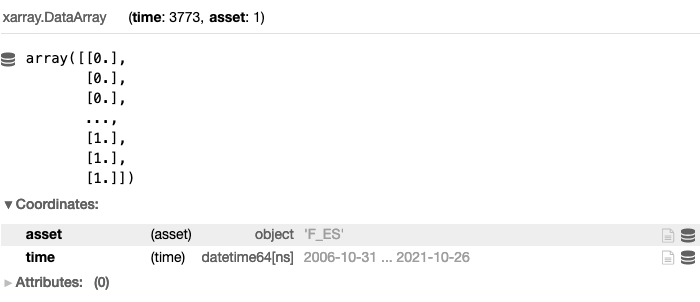
weights = qnout.clean(weights, data, 'futures')
weights
The weights xarray would look like this:
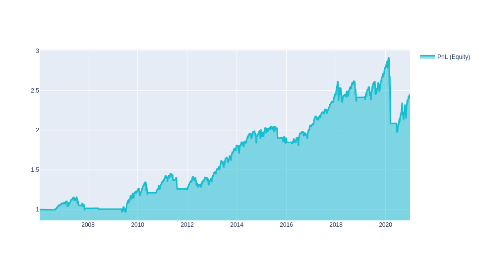
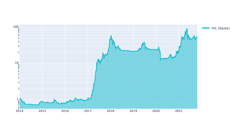
We can plot the equity chart on historical data by adding:
import qnt.stats as qnstats
import qnt.graph as qngraph

statistics = qnstats.calc_stat(data, weights)

performance = statistics.to_pandas()['equity']
qngraph.make_plot_filled(performance.index, performance, name='PnL (Equity)')
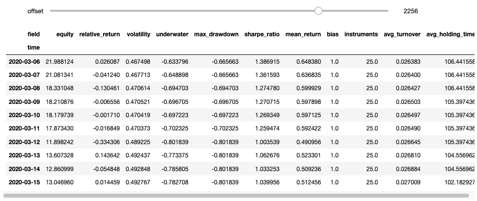
Other key statistical indicators can also be obtained by calling the calc_stat function:
equity: the cumulative value of profits and losses since inception;
relative_return: the relative daily variation of equity;
volatility: the volatility of the investment since inception (i.e. the annualized standard deviation of the daily returns);
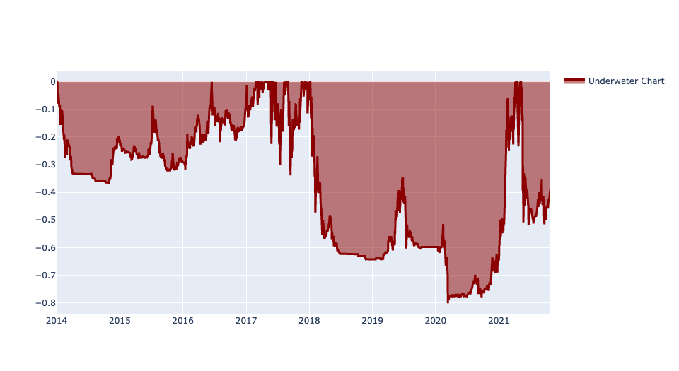
underwater: the time evolution of drawdowns;
max_drawdown: the absolute minimum of the underwater chart;
sharpe_ratio: the annualized Sharpe ratio since inception; the value must be larger than 0.7 for taking part to contests;
mean_return: the annualized mean return of the investment since inception;
bias: the daily asymmetry between long and short exposure: 1 for a long-only system, -1 for a short-only one;
instruments: the number of instruments which get allocations on a given day;
avg_turnover: the average turnover;
avg_holding_time: the average holding time in days.
All available results (indicators) can be displayed by calling:
statistics = qnstats.calc_stat(data, weights)
display(statistics.to_pandas().tail())
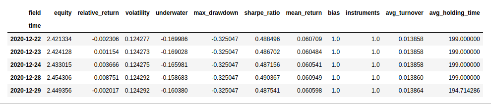
Please note that a submission needs to have an In-Sample Sharpe ratio larger than 0.7!
For a more detailed description on evaluating your algorithm with single-pass backtesting consult our API-Reference: Single-Pass Backtesting and Statistics
Multi-Pass Backtesting
For multi-pass backtesting on the other hand, you define a function that provides a set of allocation weights for the next trading day based on the entire data up to that day.
This approach actively prevents look-ahead bias issues.
Let us consider a simple long-only strategy on Cryptocurrencies: we go long once the Simple Moving Average (qnta.sma) of the close price over the last 20 trading days is larger than the Simple Moving Average of the close price over the last 200 trading days.
For this particular trading competition, which is where this example came from, it was important to only trade cryptocurrencies that were in the top 10 in market cap at the given time. Hence the weights * is_liquid step.
import xarray as xr

import qnt.ta as qnta
import qnt.backtester as qnbt
import qnt.data as qndata


def load_data(period):
    return qndata.cryptodaily_load_data(tail=period)


def strategy(data):
    close = data.sel(field='close')
    is_liquid = data.sel(field='is_liquid') # this field tags cryptocurrencies which, at a given point in time,
                                            # are among the 10 ones with the largest market capitalization
    sma_slow = qnta.sma(close, 200).isel(time=-1)
    sma_fast = qnta.sma(close, 20).isel(time=-1)
    weights  = xr.where(sma_slow < sma_fast, 1, 0) # weights only for one trading day
    weights  = weights * is_liquid  # trade only cryptocurrencies which were among the top 10 in terms
                                   # of market capitalization at each point in time
    weights = weights / 10.0
    return weights


weights = qnbt.backtest(
    competition_type= 'crypto_daily_long',
    load_data= load_data,
    lookback_period= 365,
    start_date= '2014-01-01',
    strategy= strategy
)
The backtesting runs when you call qnbt.backtest(). After it finishes, you get statistics and graphs, including:
it automatically checks the sharpe ratio:
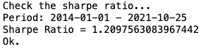
Please note that a submission needs to have an In-Sample Sharpe ratio larger than 0.7!
it shows key statistics for each day in a slidable interface:
it also visualizes different charts automatically, for example equity and underwater:
For a more detailed description on evaluating your algorithm with multi-pass backtesting consult our API-Reference: Multi-Pass Backtesting and Statistics