Financial data
Quantiacs provides historical data for the world’s major financial markets. The dataset currently includes stocks, futures (including Bitcoin futures) and cryptocurrencies. This section gives an overview of the data and documents each set:
Stocks
Quantiacs provides historic, split-adjusted data for more than 250 stocks that have been NASDAQ 100 index constituents at some point since 2001 (the beginning of index membership data). Most of these stocks are still active, but some are not. Delisted stocks are kept in the dataset to avoid survivorship bias.
Stocks list
To get the list of available stocks, use the load_ndx_list() method. By default, without any arguments, it returns stock objects (dictionaries) that have been index members in the last 4 years (default: tail=4*365). To filter the list to a specific period, pass the appropriate values:
min_date - filters the list from specific date (string, ‘yyyy-mm-dd’ format)
max_date - end date of a period, last date
tail - number of days to lookback in history from now (int)
So, call for stocks list of NASDAQ100 index members from 2006. will look:
import qnt.data as qndata
stocks_list = qndata.stocks.load_ndx_list(min_date='2006-01-01')
len(stocks_list)

231
stocks_list[:3]

[{'name': 'American Airlines Group',
  'sector': 'Consumer Goods',
  'symbol': 'AAL',
  'exchange': 'NAS',
  'id': 'NAS:AAL',
  'FIGI': 'tts-67645939'},
 {'name': 'Apple',
  'sector': 'IT/Telecommunications',
  'symbol': 'AAPL',
  'exchange': 'NAS',
  'id': 'NAS:AAPL',
  'FIGI': 'tts-831814'},
 {'name': 'Airbnb Inc',
  'sector': None,
  'symbol': 'ABNB',
  'exchange': 'NAS',
  'id': 'NAS:ABNB',
  'FIGI': 'tts-207966789'}]
You can use the additional information from the list for further filtering, such as the sector a stock belongs to. Here are a few simple functions related to sectors. First, to get the list of sectors:
def get_sectors():
    return {x['sector'] for x in stocks_list}
get_sectors()

{'Commodities',
 'Consumer Goods',
 'Energy',
 'Finance',
 'Healthcare',
 'IT/Telecommunication',
 'Industry',
 None,
 'Utilities'}
or simply, to check stocks distribution between sectors:
def sector_distribution():
    dist = dict()
    for stock in stocks_list:
        sector = stock["sector"]
        if sector not in dist:
            dist[sector] = 0
        dist[sector] += 1
    return dist
or just to get the list of symbols from specific sector:
def get_sector_stocks(sector):
    return [x['id'] for x in stocks_list if x['sector'] == sector]
like “Energy” sector:
get_sector_stocks("Energy")

['NAS:AEP', 'NAS:EXC', 'NAS:FSLR', 'NAS:PTEN', 'NAS:XEL']
finally, output is passed further to specify the set of assets for which we want to obtain data, described in next section.
Load stocks dataset
For each stock in the stocks list, you can get historical data. Use the load_ndx_data() method to load data. You can slice by time using the same parameters as load_ndx_list (min_date, tail, max_date), and also limit the result to particular assets (e.g. from a specific sector).
import qnt.data as qndata
stocks_data = qndata.stocks.load_ndx_data(min_date='2006-01-01', dims=('time', 'field', 'asset'))
stocks_data is 3-dimenional xarray structure with coordinates:
time: series of dates in string format ‘yyyy-mm-dd’
asset: list of instruments in string format, combination of first 3 characters of stock exchange and ticker symbol
field: attribute in End of Day quality
| Data field | Description |
|---|---|
| OHLC | open, high, low, close daily price |
| vol | Daily trading volume (number of shares). |
| divs | Dividend payment |
| is_liquid | The asset is NASDAQ100 constituent at that moment |
Accessing specific field, timestamp or asset from stocks_data DataArray is possible with .sel method. Let’s say we want to use only Apple data from dataset:
aapl = stocks_data.sel(asset="NAS:AAPL")
### we can convert xarray.DataArray to pandas Dataframe
aapl.to_pandas()
For more about xarray please check User Guide xarray.
Data visualization
Using the Apple data already defined as aapl above, we can create a plot for the period 2015-2020 with the plotly library:
aapl = aapl.sel(time=slice("2015-01-01", "2020-12-31")).to_pandas()
import plotly.graph_objs as go
from plotly.subplots import make_subplots


aapl_bars = make_subplots(specs=[[{"secondary_y": True}]])
aapl_bars.add_trace(go.Candlestick(x=aapl.index,
                              open=aapl['open'],
                              high=aapl['high'],
                              low=aapl['low'],
                              close=aapl['close'],
                              name='Price'))
aapl_bars.update_layout(xaxis_rangeslider_visible=False)
aapl_bars.show()
Futures
Quantiacs provides data for 78 liquid global futures contracts. The underlying assets are commodities (energy, metals, agricultural goods) and financial assets: stock indices, bonds and currency rates. In addition it provides the Bitcoin futures contract, whose history is extended back in time by patching the futures data with the Bitcoin spot data.
List of futures
The information about available futures contracts can be obtained using:
import qnt.data as qndata
future_list = qndata.futures.load_list()
future_list
The command returns a list with all available futures contracts, with their identifying symbols and full names:
[{'id': 'F_AE',
  'name': 'AEX Index',
  'sector': 'Index',
  'point_value': 'EUR 200'},
  ...,
  {'id': 'F_ES',
   'name': 'S&P 500 ETF TRUST ETF',
   'sector': 'Index',
   'point_value': '1'}]
Using the data
Suppose we want the data for the last 15 years:
import qnt.data as qndata

futures_data = qndata.futures.load_data(tail = 365*15, dims = ('time', 'field', 'asset'))
futures_data
The variable futures_data is an xarray.DataArray structure whose coordinates are:
time: a date in format yyyy-mm-dd;
asset: the identifying symbol for the asset, for example F_BP for the British Pound/US Dollar ratio.
field: an attribute, for example the opening daily price;
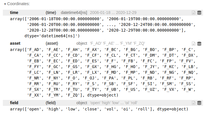
Specific fields are given by:
| Data field | Description |
|---|---|
| open | Opening daily price. |
| close | Closing daily price. |
| high | Highest daily price. |
| low | Lowest daily price. |
| vol | Daily trading volume (number of contracts). |
| oi | Total number of outstanding contracts. |
| roll | Futures contract rollover information. |
More details on xarray can be found at User Guide xarray
An example of accessing the daily open prices for each asset:
futures_data.sel(field='open')
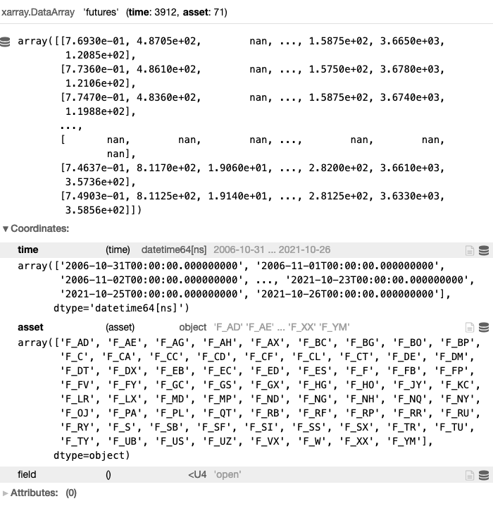
All specific fields can be accessed this way.
Values for specific contracts can be obtained selecting the asset. Let us say we are interested in British pound futures. We can get the close price as follows:
GBP_USD = futures_data.sel(asset = 'F_BP').sel(field = 'close')
For a more detailed description on loading and accessing Futures data consult our API-Reference: Loading Futures Data
For visualizing the data we can use for example the plotly library https://plotly.com/:
import plotly.graph_objs as go

trend_fig = [go.Scatter(
    x = GBP_USD.to_pandas().index,
    y = GBP_USD,
    line = dict(width=1, color='black'))]

fig = go.Figure(data = trend_fig)
fig.update_yaxes(fixedrange=False)
fig.show()
Using the BTC futures
For a more detailed description on loading and accessing BTC futures, see the API reference: Loading BTC Futures Data
The Bitcoin Futures data for the last 8 years (history extended with Bitcoin spot price) can be loaded using:
import qnt.data as qndata

btc_data = qndata.cryptofutures.load_data(tail = 365*8, dims = ('time', 'field', 'asset'))
Front contracts and different maturity contracts
As several Futures contracts with the same underlying instrument but different expiration dates (maturities) are traded on financial exchange at the same time, we provide the option to load continuous front contracts (closest expiration date), next-to-front contracts (next-to-closest expiration date) and next-to-next-to-front contracts (next-to-next-to-closest expiration date):
front_data                 = qndata.futures.load_data(min_date='1900-01-01', offset=0)
next_to_front_data         = qndata.futures.load_data(min_date='1900-01-01', offset=1)
next_to_next_to_front_data = qndata.futures.load_data(min_date='1900-01-01', offset=2)
Note that the default choice (no offset specified) selects front contracts. All three options are continuous contracts, obtained by patching together the single Futures contracts.
All three continuous contracts can be used as indicators, but only the front contracts will be used for the backtesting and real trading.
Spot currency data
Currency rates taken from the International Monetary Fund page can be inspected using:
import pandas as pd
import qnt.data as qndata
currency_list = qndata.imf_load_currency_list()
pd.DataFrame(currency_list)
which returns the list for 39 time series:

Data for each time series can be loaded using (for example last 5 years):
euro_currency = qndata.imf_load_currency_data(assets=['EUR'], tail=365 * 5)
Spot commodity data
Commodity data taken from the International Monetary Fund page can be inspected using:
import pandas as pd
import qnt.data as qndata
commodity_list = qndata.imf_load_commodity_list()
pd.DataFrame(commodity_list)
which returns the list for 76 time series:
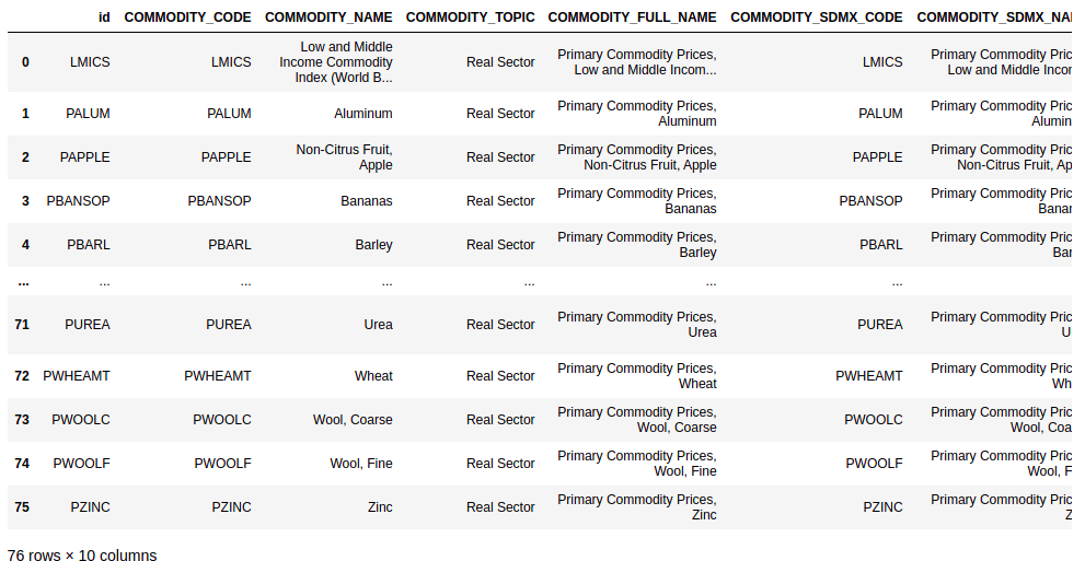
Data for each time series can be loaded using (for example last year):
gold = qndata.imf_load_commodity_data(assets=['PGOLD'], tail=365)
Cryptocurrencies
Cryptocurrency daily data
Quantiacs provides up-to-date daily data for 54 cryptocurrencies:
['ADA', 'AUR', 'AVAX', 'BCH', 'BCN', 'BLK', 'BNB', 'BSV', 'BTC', 'BTG',
   'BTS', 'DASH', 'DGC', 'DGD', 'DOGE', 'DOT', 'EOS', 'ETC', 'ETH', 'FCT',
   'FRC', 'FTC', 'GNT', 'ICP', 'IFC', 'IXC', 'LINK', 'LSK', 'LTC', 'MAID',
   'MNC', 'NEO', 'NMC', 'NXT', 'OMNI', 'PPC', 'QRK', 'REP', 'SOL', 'STEEM',
   'STRAX', 'THETA', 'TRC', 'TRX', 'UNI', 'WAVES', 'WDC', 'XCP', 'XEM',
   'XLM', 'XMR', 'XPM', 'XPY', 'XRP']
The available cryptocurrency data for the last 5 years can be loaded using:
import qnt.data as qndata

crypto_data = qndata.cryptodaily.load_data(tail = 365 * 5)
For each cryptocurrency data is available on an daily resolution. crypto_data is an xarray.DataArray structure whose coordinates are:
time: a date-time in format yyyy-mm-dd;
asset: the identifying symbol for the asset, for example ETH for Ethereum.
field: an attribute, for example the opening hourly price;
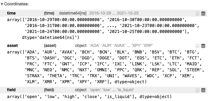
Specific fields are given by:
| Data field | Description |
|---|---|
| open | Opening daily price. |
| close | Closing daily price. |
| high | Highest daily price. |
| low | Lowest daily price. |
| is_liquid | Is this cryptocurrency liquid? |
For a more detailed description on loading and accessing Crypto Daily data consult our API-Reference: Loading Crypto Daily Data
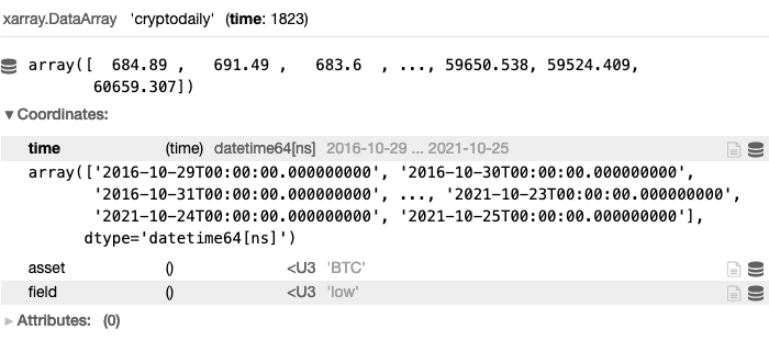
Let us say we are interested in the lowest daily price for BTC. We can extract it using:
crypto_data.sel(field = 'low').sel(asset = 'BTC')
Cryptocurrency hourly data
Quantiacs provides up-to-date hourly data - price and volume - for the following cryptocurrencies:
Bitcoin (BTC);
Bitcoin Cash (BCH);
EOS;
Ethereum (ETH);
Litecoin (LTC);
Ripple (XRP);
Tether (USDT).
The available cryptocurrency data for the last 5 years can be loaded using:
import qnt.data as qndata

crypto_data = qndata.crypto.load_data(tail = 365 * 5)
For each cryptocurrency data are available on an hourly resolution. crypto_data is an xarray.DataArray structure whose coordinates are:
time: a date-time in format yyyy-mm-ddTHH-MM-SS;
asset: the identifying symbol for the asset, for example ETH for Ethereum;
field: an attribute, for example the opening hourly price;

Specific fields are given by:
| Data field | Description |
|---|---|
| open | First price in a given hour. |
| close | Last price in a given hour. |
| high | Highest price in a given hour. |
| low | Lowest price in a given hour. |
| vol | Hourly trading volume. |
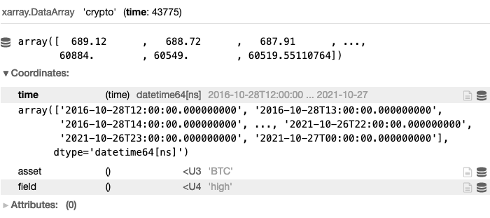
Let us say we are interested in the highest hourly price for BTC. We can extract it using:
BTC_high = crypto_data.sel(field = 'high').sel(asset = 'BTC')
BTC_high
The BTC_high data can then be visualized using:
import plotly.graph_objs as go

trend_fig = [go.Scatter(
    x = BTC_high.to_pandas().index,
    y = BTC_high,
    line = dict(width=1,color='black'))]

fig = go.Figure(data = trend_fig)
fig.update_yaxes(fixedrange=False)
fig.show()
For a more detailed description on loading and accessing Crypto Hourly data consult our API-Reference: Loading Crypto Hourly Data